张量的线性代数运算
- pytorch中BLAS和LAPACK模块的相关运算
- pytorch中没有设置单独的矩阵对象类型,因此,在pytorch中二维张量就相当于矩阵对象,并且拥有一系列线性代数相关函数和方法
1
2
| import torch
import numpy as np
|
一、BLAS和LAPACK概览
- 矩阵的新编及特殊矩阵的构造方法:包括矩阵的转置、对角矩阵的创建、单位矩阵的创建、上/下三角矩阵的创建等;
- 矩阵的基本运算:矩阵乘法、向量內积、矩阵和向量的乘法等
- 矩阵的线性代数运算:包括矩阵的迹、矩阵的秩、逆矩阵的求解、伴随矩阵和广义逆矩阵等
- 矩阵分解运算:特征分解、奇异值分解和SVD分解等
二、矩阵的形态及特殊矩阵构造方法
| 函数 |
描述 |
| torch.t(t) |
t转置 |
| torch.eye(n) |
创建包含n个分量的单位矩阵 |
| torch.diag(t1) |
以t1中各元素创建对角矩阵 |
| torch.triu(t) |
去矩阵t中上三角矩阵 |
| torch.tril(t) |
去矩阵t中下三角矩阵 |
1
2
| t1=torch.arange(1,7).reshape(2,3).float()
t1
|
tensor([[1., 2., 3.],
        [4., 5., 6.]])
tensor([[1., 4.],
        [2., 5.],
        [3., 6.]])
tensor([[1., 4.],
        [2., 5.],
        [3., 6.]])
tensor([[1., 0., 0.],
        [0., 1., 0.],
        [0., 0., 1.]])
1
2
| t=torch.arange(5)
torch.diag(t)
|
tensor([[0, 0, 0, 0, 0],
        [0, 1, 0, 0, 0],
        [0, 0, 2, 0, 0],
        [0, 0, 0, 3, 0],
        [0, 0, 0, 0, 4]])
1
2
| t1=torch.arange(9).reshape(3,3)
torch.triu(t1)
|
tensor([[0, 1, 2],
        [0, 4, 5],
        [0, 0, 8]])
tensor([[0, 0, 0],
        [3, 4, 0],
        [6, 7, 8]])
tensor([[0, 1, 2],
        [3, 4, 5],
        [0, 7, 8]])
tensor([[0, 1, 2],
        [0, 0, 5],
        [0, 0, 0]])
三、矩阵的基本运算
| 函数 |
描述 |
| torch.dot(t1,t2) |
计算t1、t2张量內积 |
| torch.mm(t1,t2) |
矩阵乘法 |
| torch.mv(t1,t2) |
矩阵乘向量 |
| torch.bmm(t1,t2) |
批量矩阵乘法 |
| torch.addmm(t,t1,t2) |
矩阵相乘后相加 |
| torch.addbmm(t,t1,t2) |
批量矩阵相乘后相加 |
- dot\vdot:点积计算
在pytorch中,dot和vdot只能作用于一维张量,对于数值型对象,二者计算结果没有区别,在复数运算时有区别
tensor([1, 2, 3])
tensor(14)
tensor(14)
1
2
| t1=torch.arange(1,7).reshape(2,3)
t1
|
tensor([[1, 2, 3],
[4, 5, 6]])
1
2
| t2=torch.arange(1,10).reshape(3,3)
t2
|
tensor([[1, 2, 3],
[4, 5, 6],
[7, 8, 9]])
tensor([[ 1, 4, 9],
[16, 25, 36]])
tensor([[30, 36, 42],
[66, 81, 96]])
- mv:矩阵和向量相乘
先将向量转为列向量然后再相乘
1
2
| met=torch.arange(1,7).reshape(2,3)
met
|
tensor([[1, 2, 3],
        [4, 5, 6]])
1
2
| vec=torch.arange(1,4)
vec
|
tensor([1, 2, 3])
tensor([14, 32])
tensor([[1],
[2],
[3]])
1
| torch.mm(met,vec.reshape(3,1))
|
tensor([[14],
[32]])
1
| torch.mm(met,vec.reshape(3,1)).flatten()
|
tensor([14, 32])
mv函数本质上提供了一种二维张量和一维张量相乘的方法,再线性代数运算过程中,有很多矩阵乘向量的场景,典型的如线性回归的求解过程,通常情况下我们需要将向量转化位列向量然后进行计算,但pytorch中单独设置了一个矩阵和向量相乘的方法,从而简化了行/列向量的理解过程和将向量转为列向量的转化过程
- bmm:批量矩阵相乘
指三维张量的矩阵乘法,三维张量内各对应位置的矩阵相乘
1
2
| t3=torch.arange(1,13).reshape(3,2,2)
t3
|
tensor([[[ 1, 2],
[ 3, 4]],
[[ 5, 6],
[ 7, 8]],
[[ 9, 10],
[11, 12]]])
1
2
| t4=torch.arange(1,19).reshape(3,2,3)
t4
|
tensor([[[ 1, 2, 3],
[ 4, 5, 6]],
[[ 7, 8, 9],
[10, 11, 12]],
[[13, 14, 15],
[16, 17, 18]]])
tensor([[[ 9, 12, 15],
[ 19, 26, 33]],
[[ 95, 106, 117],
[129, 144, 159]],
[[277, 296, 315],
[335, 358, 381]]])
point:
- 三维张量包含的矩阵个数需要相同
- 每个内部矩阵,需要满足矩阵乘法的条件,ab bc -> ac
- addmm:矩阵相乘后相加
addmm函数结构:addmm(input,mat1,mat2,beta=1,alpha=1)
输出结果:beta*input+alpha*(mat1*mat2)
tensor([[1, 2, 3],
[4, 5, 6]])
tensor([[1, 2, 3],
        [4, 5, 6],
        [7, 8, 9]])
tensor([0, 1, 2])
tensor([[30, 36, 42],
        [66, 81, 96]])
tensor([[30, 37, 44],
[66, 82, 98]])
1
| torch.addmm(t,t1,t2,beta=0,alpha=10)
|
tensor([[300, 360, 420],
[660, 810, 960]])
四、矩阵的线性代数运算
| 函数 |
描述 |
| torch.trace(A) |
矩阵的迹 |
| matrix_rank(A) |
矩阵的秩 |
| torch.det(A) |
计算矩阵A的行列式 |
| torch.inverse(A) |
矩阵求逆 |
| torch.lstsq(A,B) |
最小二乘法 |
- 矩阵的迹(trace)
矩阵的迹就是计算矩阵对角线元素之和
1
2
| A=torch.tensor([1,2,4,5]).reshape(2,2).float()
A
|
tensor([[1., 2.],
[4., 5.]])
tensor(6.)
1
2
| B=torch.arange(1,7).reshape(2,3)
B
|
tensor([[1, 2, 3],
        [4, 5, 6]])
tensor(6)
- 矩阵的秩(rank)
矩阵的秩是指矩阵中行或列的极大线性无关组个数,矩阵的秩唯一
1
2
| A=torch.arange(1,5).reshape(2,2).float()
A
|
tensor([[1., 2.],
[3., 4.]])
tensor(2)
1
2
| B=torch.tensor([[1,2],[2,4]]).float()
B
|
tensor([[1., 2.],
[2., 4.]])
tensor(1)
- 矩阵的行列式(det)
行列式作为一个基本数学工具,实际上就是进行线性变换的伸缩因子
对于任何一个n维方阵,行列式的计算过程如下:
D=∣∣∣∣∣∣∣∣∣a11a21⋯an1a12a22⋯an2⋯⋯⋯⋯a1na2n⋯ann∣∣∣∣∣∣∣∣∣
D=∑(−1)ka1k1a2k2⋯ankn
对于一个2*2的矩阵,行列式的计算就是主对角线元素之积减去另外两个元素之积
1
2
| A=torch.tensor([[1,2],[4,5]]).float()
A
|
tensor([[1., 2.],
[4., 5.]])
tensor(-3.)
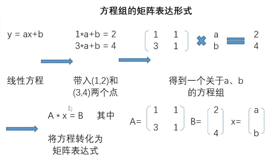
- 线性方程组的矩阵表达形式
矩阵-》由向量组组成的矩阵
1
2
| A=torch.arange(1,5).reshape(2,2).float()
A
|
tensor([[1., 2.],
[3., 4.]])
1
2
| import matplotlib as mpl
import matplotlib.pyplot as plt
|
1
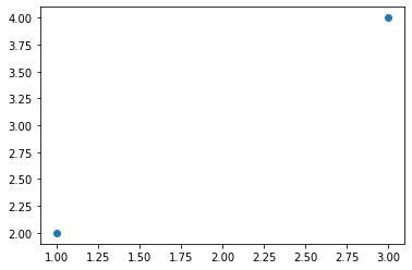
| plt.plot(A[:,0],A[:,1],'o')
|
[<matplotlib.lines.Line2D at 0x22856f5ae80>]
![image]()
如果更进一步,我们希望在二维空间中找到一条直线,来拟合这两个点,也就是构建一个线性回归模型,我们可以设置线性回归方程如下:
y=ax+b
带入(1,2)和(3,4)两个点后,我们还可以进一步将表达式改写成矩阵表示形式。
A*x=B
![image]()
1
2
| A=torch.tensor([[1.0,1],[3,1]])
A
|
tensor([[1., 1.],
[3., 1.]])
1
2
| B=torch.tensor([2.0,4])
B
|
tensor([2., 4.])
tensor([[-0.5000, 0.5000],
[ 1.5000, -0.5000]])
1
| torch.mm(torch.inverse(A),A)
|
tensor([[ 1.0000e+00, -5.9605e-08],
[-1.1921e-07, 1.0000e+00]])
x=A−1∗B
1
| torch.mv(torch.inverse(A),B)
|
tensor([1.0000, 1.0000])
a=1,b=1
最终得到线性方程为y=x+1
五、矩阵的分解
矩阵的分解也是矩阵运算中常规计算,矩阵分解有很多种类,常见的例如QR分解、LU分解、特征分解和SVD分解,虽然大多数情况下,矩阵分解都是在形式上将矩阵拆分成几种特殊矩阵的乘积。分解之后的等式如下:
A=V∪D
- 特征分解
特征分解中,矩阵分解形式为:
A=QΛQ−1
其中Q和Q−1互为逆矩阵,Q的列就是A的特征值对应的特征向量,Λ就是特征值组成的对角矩阵
1
2
| A=torch.arange(1,10).reshape(3,3).float()
A
|
tensor([[1., 2., 3.],
[4., 5., 6.],
[7., 8., 9.]])
1
| torch.eig(A,eigenvectors=True)
|
torch.return_types.eig(
eigenvalues=tensor([[ 1.6117e+01, 0.0000e+00],
[-1.1168e+00, 0.0000e+00],
[ 2.9486e-07, 0.0000e+00]]),
eigenvectors=tensor([[-0.2320, -0.7858, 0.4082],
[-0.5253, -0.0868, -0.8165],
[-0.8187, 0.6123, 0.4082]]))
- 奇异值分解(SVD)
奇异值分解是特征值分解在奇异矩阵上的推广形式,它将一个维度为mxn的奇异矩阵A分解为三个部分:
A=U∑VT
其中U、V是两个正交矩阵,其中的每一行(列)分别被称为左奇异向量和右奇异向量,他们和∑中对角线上的奇异值相对应,通常情况下我们只保留前k和奇异向量和奇异值。其中U是mxk矩阵,V是nxk矩阵,∑是kxk的方阵,从而减少存储空间的效果
Am∗n=Um∗nm∗n∑Vn∗nT≈Um∗kk∗k∑Vk∗nT
1
2
| C=torch.tensor([[1., 2., 3.],[2., 4., 6.],[3., 6., 9.]])
C
|
tensor([[1., 2., 3.],
[2., 4., 6.],
[3., 6., 9.]])
torch.return_types.svd(
U=tensor([[-2.6726e-01, 9.6362e-01, -3.7767e-08],
[-5.3452e-01, -1.4825e-01, -8.3205e-01],
[-8.0178e-01, -2.2237e-01, 5.5470e-01]]),
S=tensor([1.4000e+01, 4.2751e-08, 1.6397e-15]),
V=tensor([[-0.2673, -0.9636, 0.0000],
[-0.5345, 0.1482, -0.8321],
[-0.8018, 0.2224, 0.5547]]))
tensor([[1.4000e+01, 0.0000e+00, 0.0000e+00],
[0.0000e+00, 4.2751e-08, 0.0000e+00],
[0.0000e+00, 0.0000e+00, 1.6397e-15]])
1
| torch.mm(torch.mm(CU,torch.diag(CS)),CV.t())
|
tensor([[1.0000, 2.0000, 3.0000],
[2.0000, 4.0000, 6.0000],
[3.0000, 6.0000, 9.0000]])
能够看出,上述输出完成还原了C矩阵,此时我们可根据svd输出结果对C进行降维,此时C可只保留第一列,即k=1
1
2
| U1=CU[:,0].reshape(3,1)
U1
|
tensor([[-0.2673],
[-0.5345],
[-0.8018]])
tensor(14.0000)
1
2
| V1=CV[:,0].reshape(1,3)
V1
|
tensor([[-0.2673, -0.5345, -0.8018]])
tensor([[1.0000, 2.0000, 3.0000],
        [2.0000, 4.0000, 6.0000],
        [3.0000, 6.0000, 9.0000]])
此时输出的Cd矩阵以及和原矩阵高度相似了,损失信息在R的计算中基本可以忽略不计,经过SVD分解,矩阵的信息能够被压缩至更小的空间内进行存储,从而为PCA(主成分分析)、LSI(潜在语义索引)等算法做好了数学工具层面的铺垫